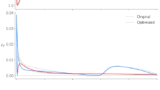
pymooのNSGA-IIとxfoilでCST Airfoilの多目的最適化を行う
xfoilを使うため、pythonのバージョンは3.6、pymooのバージョンは0.5.0である(結果の可視化のために.gifのアニメーションを作るときはpython 3.10を使う)

はじめに
pymooのNSGA-IIとxfoilでCST Airfoilの多目的最適化を行う
最終的にはこんな感じになる
↓公式ドキュメント


↓参考
ちなみに、今回使う多目的最適化のアルゴリズム「NSGA-II」の詳しい原理についてはノリでしか理解していない
↓xfoilのインストール
それではいってみよう
使い方
ソースコードはこれ
https://github.com/mtkbirdman/mtkbirdman.com/blob/master/MDO/NSGA2.pyfrom CST import CST
import sys
import time
import numpy as np
import pandas as pd
from xfoil import XFoil
from xfoil.model import Airfoil
from ctypes import cdll
from pymoo.util.misc import stack
from pymoo.core.problem import Problem
from pymoo.algorithms.moo.nsga2 import NSGA2
from pymoo.operators.sampling.lhs import LHS
from pymoo.operators.crossover.sbx import SBX
from pymoo.operators.mutation.pm import PolynomialMutation
#from pymoo.termination import get_termination # pymoo==0.6.0
from pymoo.optimize import minimize
from pymoo.visualization.scatter import Scatter
# Create an instance of the XFoil class for airfoil analysis
xf = XFoil()
# Define a custom optimization problem
class MyProblem(Problem):
def __init__(self, file_name='airfoil_shape.csv', n_wu=4, n_wl=4, x_diff=0.8):
self.n_wu = n_wu # Number of control points for the upper surface
self.n_wl = n_wl # Number of control points for the lower surface
# Create an instance of the CST class for airfoil parameterization
airfoil = CST()
airfoil.fit_CST(file_name=file_name, n_wu=self.n_wu, n_wl=self.n_wl)
# Retrieve airfoil properties
self.thickness, self.x_tmax = airfoil.get_thickness()
self.ler = airfoil.get_ler()
self.TE_angle = airfoil.get_TE_angle()
self.section_area = airfoil.get_section_area()
self.w_LE = np.abs(np.abs(airfoil.wu[0,0])-np.abs(airfoil.wl[0,0]))
# Initial guess for the design variables
x0 = np.concatenate([airfoil.wu, airfoil.wl], axis=1).reshape(-1)
xu = x0*(1 + np.sign(x0)*x_diff) # Upper bounds for design variables
xl = x0*(1 - np.sign(x0)*x_diff) # Lower bounds for design variables
super().__init__(n_var=self.n_wu + self.n_wl,
n_obj=2,
n_constr=6,
xl=xl,
xu=xu)
# Additional properties for airfoil analysis
self.M = 0.0 # Mach number
self.n_cirt = 9 # Critical amplification ratio
self.xtr = (1, 1) # Transition points on the upper and lower surfaces
self.max_iter = 100 # Maximum number of iterations for XFoil
self.Re = 1000000 # Reynolds number
self.cl = 0.5 # Target lift coefficient
def _evaluate(self, X, out, *args, **kwargs):
wu = X[:, 0:self.n_wu].tolist() # Upper surface control points
wl = X[:, self.n_wu:].tolist() # Lower surface control points
dz = np.zeros(X.shape[0]).reshape(-1, 1).tolist() # Zero thickness distribution
Node = 101 # Number of nodes for airfoil discretization
# Create airfoil shapes using CST
airfoil = CST()
airfoil.create_airfoil(wu=wu, wl=wl, dz=dz, Node=Node)
# Retrieve updated airfoil properties
thickness, x_tmax = airfoil.get_thickness()
ler = airfoil.get_ler()
TE_angle = airfoil.get_TE_angle()
section_area = airfoil.get_section_area()
w_LE = np.abs(np.abs(airfoil.wu[:,0])-np.abs(airfoil.wl[:,0]))
f1_list = [] # List to store drag coefficients
f2_list = [] # List to store pitching moments
g1_list = [] # List to store lift coefficients (for constraints)
for i in range(X.shape[0]):
# Calculate aerodynamic properties for each airfoil shape
f1, f2, g1 = self._calculate(airfoil=airfoil, idx=i)
f1_list.append(f1)
f2_list.append(f2)
g1_list.append(g1)
f1 = np.array(f1_list)
f2 = np.array(f2_list)
g_diff = 0.5
g1 = np.array(g1_list) # cl0 > 0
g2 = (self.thickness - thickness) / self.thickness
g3 = (w_LE-self.w_LE/g_diff) / self.w_LE
g4 = (self.section_area*g_diff - section_area) / self.section_area
g5 = (self.TE_angle*g_diff - TE_angle) / self.TE_angle
g6 = (self.ler*g_diff - ler) / self.ler
#g7 = (0.00 - x_tmax) / self.x_tmax
# Output objectives and constraints
out["F"] = np.column_stack([f1, f2])
out["G"] = np.column_stack([g1, g2, g3, g4, g5, g6]) #, g7])
def _calculate(self, airfoil, idx):
# Assign airfoil coordinates to XFoil
xf.airfoil = Airfoil(airfoil.x[idx], airfoil.y[idx])
# Define analysis parameters
xf.M = self.M # Mach number
xf.n_crit = self.n_cirt # Critical amplification ratio
xf.xtr = self.xtr # Transition points
xf.max_iter = self.max_iter # Maximum number of iterations
xf.Re = self.Re # Reynolds number
# Perform analysis with XFoil
xf.repanel() # Re-panel airfoil
a, cd, cm, cp = xf.cl(self.cl) # Analyze at fixed lift coefficient
cl0, cd0, cm0, cp0 = xf.a(0) # Analyze at zero angle of attack
xf.reset_bls() # Reset boundary layers
return cd, -cm, -cl0 # Return drag, pitching moment, and lift coefficient
if __name__ == '__main__':
# Mesure execution time
start_time = time.time()
# Define the optimization problem
problem = MyProblem(file_name='./MDO/NACA4412.csv', n_wu=5, n_wl=5, x_diff=1.5)
# Initialize the NSGA-II algorithm
algorithm = NSGA2(
pop_size=100,
#n_offsprings=10,
sampling=LHS(), # Latin Hypercube Sampling
crossover=SBX(prob=0.9, eta=15), # Simulated Binary Crossover
mutation=PolynomialMutation(eta=20), # Polynomial Mutation
eliminate_duplicates=True
)
# Termination criterion (optional)
#termination = get_termination("n_gen", 40) # pymoo==0.6.0
# Execute the optimization
res = minimize(
problem,
algorithm,
#termination, # pymoo==0.6.0
("n_gen", 100), # Number of generations
seed=1, # Random seed for reproducibility
save_history=True,
verbose=True
)
# Save optimization results
pd.DataFrame(res.X).to_csv('./MDO/res_X.csv', index=False)
pd.DataFrame(res.F, columns=['cd', 'cm']).to_csv('./MDO/res_F.csv', index=False)
pd.DataFrame(res.G, columns=['cl0', 't/c', 'w_LE', 'section_area', 'TE_angle', 'ler']).to_csv('./MDO/res_G.csv', index=False)
#pd.DataFrame(res.G, columns=['cl0', 't/c', 'w_LE', 'section_area', 'TE_angle', 'ler', 'x_tmax', ]).to_csv('./MDO/res_G.csv', index=False)
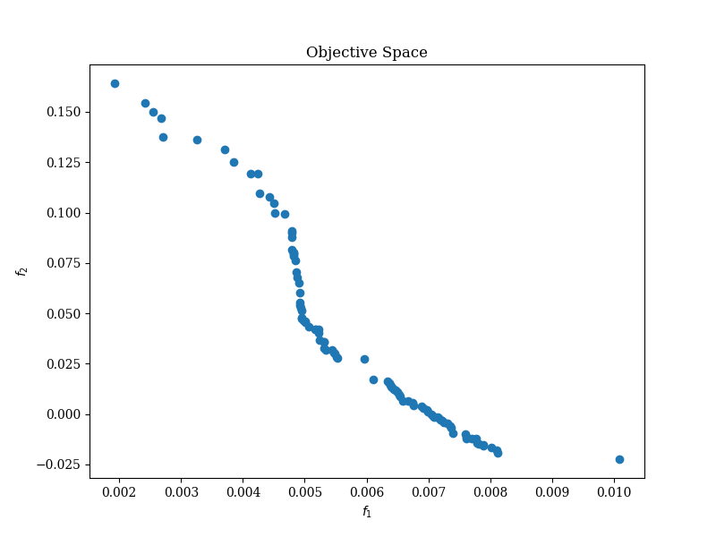
# Plot the objective space
plot = Scatter(title="Objective Space")
plot.add(res.F)
plot.show()
end_time = time.time()
print(f"Run time: {end_time - start_time} s")
NSGA2.py、ベースとなる翼型データの.csvファイル、および後述するCST.pyを同じディレクトリにおいて、以下のコマンドを実行する
py -3.6 NSGA2.pyxfoilの標準出力が鬼のように流れるので、しばらく放置しておく(FORTRANで書かれた外部ライブラリの標準出力の止め方が分からなかった...)
筆者の環境での実行時間は以下の通り
| 設計変数の数 | 個体数 | 世代数 | 実行時間 [s] |
| 10 | 50 | 50 | 912.754 |
| 10 | 100 | 50 | 2074.124 |
| 10 | 50 | 100 | 1973.023 |
| 10 | 100 | 100 | 2571.368 |
下のグラフが表示されたら最適化が終了している
最初に示した.gifファイルを作るには、check.pyを実行する
https://github.com/mtkbirdman/mtkbirdman.com/blob/master/MDO/check.pyfrom CST import CST # CSTモジュールからCSTクラスをインポート
import sys
import numpy as np
import pandas as pd
import matplotlib.pyplot as plt
import matplotlib.animation as animation
def _update_left(i, ax_left, res, airfoil):
"""
左側のプロットを更新する関数
Args:
- i: 現在のフレーム番号
- ax_left: 左側のプロットの軸オブジェクト
- res: 最適化結果のデータフレーム
- airfoil: 翼型形状データ
"""
ax_left.clear() # 現在描写されているグラフを消去
ax_left.set_title("cd = {:.4f} cm = {:.4f}".format(res['cd'].iloc[i], -res['cm'].iloc[i])) # タイトルに現在のcdとcmの値を表示
ax_left.set_xlim(0, 1) # x軸の範囲を設定
ax_left.set_ylim(-0.5, 0.5) # y軸の範囲を設定
ax_left.plot(airfoil.x[i], airfoil.y[i], color='blue') # 翼型形状をプロット
def _update_right(i, ax_right, res):
"""
右側のプロットを更新する関数
Args:
- i: 現在のフレーム番号
- ax_right: 右側のプロットの軸オブジェクト
- res: 最適化結果のデータフレーム
"""
ax_right.clear() # 現在描写されているグラフを消去
ax_right.set_title('cd vs cm') # タイトルを設定
ax_right.set_ylim(0, 0.012) # y軸の範囲を設定
ax_right.set_xlim(-0.1, 0.02) # x軸の範囲を設定
ax_right.set_xticks([-0.20, -0.16, -0.12, -0.08, -0.04, 0.00, 0.04]) # x軸のメモリを設定
ax_right.set_ylabel('cd') # y軸のラベルを設定
ax_right.set_xlabel('cm') # x軸のラベルを設定
ax_right.grid() # グリッドを表示
ax_right.plot(-res['cm'], res['cd'], '.', color='blue') # cd vs cmのプロット
ax_right.plot(-res['cm'].values[i], res['cd'].values[i], '*', color='red', markersize=10) # 現在のフレームのデータを強調表示
def gif_animation(res, airfoil):
"""
GIFアニメーションを作成する関数
Args:
- res: 最適化結果のデータフレーム
- airfoil: 翼型形状データ
"""
fig, (ax_left, ax_right) = plt.subplots(1, 2, figsize=(12, 6)) # 左右に2つのプロットを持つ図を作成
def _update(i):
_update_left(i, ax_left, res, airfoil) # 左側のプロットを更新
_update_right(i, ax_right, res) # 右側のプロットを更新
ani = animation.FuncAnimation(fig, _update, interval=100, frames=len(res), repeat_delay=2000) # アニメーションを作成
# 保存
ani.save("./MDO/sample.gif", writer="pillow") # アニメーションをGIFとして保存
def objective_space(res):
"""
目的空間のプロットを表示する関数
Args:
- res: 最適化結果のデータフレーム
"""
fig = plt.figure(figsize=(6, 6)) # 図のサイズを指定して作成
plt.title('cd vs cm') # タイトルを設定
plt.ylabel('cd') # y軸のラベルを設定
plt.xlabel('cm') # x軸のラベルを設定
plt.ylim(0, 0.012) # y軸の範囲を設定
plt.xlim(-0.20, 0.04) # x軸の範囲を設定
plt.xticks([-0.20, -0.16, -0.12, -0.08, -0.04, 0.00, 0.04]) # x軸の目盛りを設定
plt.grid() # グリッドを表示
plt.plot(-res['cm'], res['cd'], '.', color='blue') # cd vs cmのプロット
# 表示
plt.show() # プロットを表示
# 最適化結果の読み込み
res_X = pd.read_csv('./MDO/res_X.csv')
res_F = pd.read_csv('./MDO/res_F.csv')
# 結果を結合し、cdでソート
res = pd.concat([res_X, res_F], axis=1)
res = res.sort_values('cd')
res_np = res.to_numpy()
# 翼型形状を生成
airfoil = CST()
n_wu = int(res_X.shape[1]/2)
wu = res_np[:, :n_wu].tolist()
wl = res_np[:, n_wu:].tolist()
dz = np.zeros(len(wu)).tolist()
airfoil.create_airfoil(wu=wu, wl=wl, dz=dz, Node=100)
# 目的空間のプロットを表示
objective_space(res)
# GIFアニメーションを作成
gif_animation(res, airfoil)プログラム実行後、同じディレクトリにresult.gifが保存される
py -3.10 check.py↓CST.pyについて
ソースコードの解説
NSGA2.pyは、CST (Class-Shape Transformation) メソッドを用いて翼型の形状を最適化するPythonプログラムである
翼型の形状をCST Airfoilとしてパラメータ化し、NSGA-IIアルゴリズムを使用して、複数の目的関数(今回はcl=0.5における抗力係数cdおよびピッチングモーメント係数cm)に対して最適化を行う
使用ライブラリ
CST: 翼型の形状パラメータ化に使用sys,numpy,pandas: データ操作に使用xfoil: 翼型の空力解析に使用pymoo: 多目的最適化アルゴリズムに使用(バージョン0.5.0)
最初のほう
Import
from CST import CST # 自作

import sys
import time
import numpy as np
import pandas as pd

from xfoil import XFoil
from xfoil.model import Airfoil
from ctypes import cdll

from pymoo.util.misc import stack
from pymoo.core.problem import Problem
from pymoo.algorithms.moo.nsga2 import NSGA2
from pymoo.operators.sampling.lhs import LHS
from pymoo.operators.crossover.sbx import SBX
from pymoo.operators.mutation.pm import PolynomialMutation
#from pymoo.termination import get_termination # pymoo==0.6.0
from pymoo.optimize import minimize
from pymoo.visualization.scatter import Scatter- 必要なライブラリとモジュールをインポートする
XFoilのインスタンス化
xf = XFoil()- 翼型の空力解析を行うためのXFoilクラスのインスタンスを作成する
最適化問題の定義
class MyProblem(Problem):
    def __init__(self, file_name='airfoil_shape.csv', n_wu=4, n_wl=4, x_diff=0.1):
        self.n_wu = n_wu  # Number of control points for the upper surface
self.n_wl = n_wl # Number of control points for the lower surface- 最適化問題を定義するクラス
MyProblemを作成し、__init__メソッドで初期化を行う - ここでは、翼型の設計変数の範囲などを設定する
翼型の形状フィッティングとプロパティの取得
        airfoil = CST()
        airfoil.fit_CST(file_name=file_name, n_wu=self.n_wu, n_wl=self.n_wl)
        self.thickness, self.x_tmax = airfoil.get_thickness()
        self.ler = airfoil.get_ler()
        self.TE_angle = airfoil.get_TE_angle()
        self.w_LE = np.abs(np.abs(airfoil.wu[0,0])-np.abs(airfoil.wl[0,0]))
        x0 = np.concatenate([airfoil.wu, airfoil.wl], axis=1).reshape(-1)
        xu = x0*(1 + np.sign(x0)*x_diff)  # Upper bounds for design variables
xl = x0*(1 - np.sign(x0)*x_diff) # Lower bounds for design variables- ベース翼型の形状をCSTメソッドでフィッティングし、翼厚、前縁半径、後縁角度などのプロパティを取得する
- ベース翼型のCSTパラメータをもとに、最適化の際にCSTパラメータがとりうる範囲を設定する(
x_diffの大きさの設定はパラメータ職人の腕の見せ所)
問題の定義
        super().__init__(n_var=self.n_wu + self.n_wl,
                         n_obj=2,
                         n_constr=6,
                         xl=xl,
xu=xu)- 親クラスである
Problemクラスの初期化メソッドをsuper()で呼び出し、設計変数の数、目的関数の数、制約条件の数、および設計変数の範囲(上限と下限)を設定する
xfoilのプロパティ設定
        self.M = 0.0  # Mach number
        self.n_cirt = 9  # Critical amplification ratio
        self.xtr = (1, 1)  # Transition points on the upper and lower surfaces
        self.max_iter = 100  # Maximum number of iterations for XFoil
        self.Re = 1000000  # Reynolds number
self.cl = 0.5 # Target lift coefficient- xfoilの空力解析に必要な追加のプロパティ(マッハ数、遷移点、最大反復回数、レイノルズ数、目標揚力係数)を設定する
評価関数の定義
    def _evaluate(self, X, out, *args, **kwargs):
        wu = X[:, 0:self.n_wu].tolist()  # Upper surface control points
        wl = X[:, self.n_wu:].tolist()  # Lower surface control points
        dz = np.zeros(X.shape[0]).reshape(-1, 1).tolist()  # Zero thickness distribution
Node = 201 # Number of nodes for airfoil discretization_evaluateメソッドで、目的関数の定義を行う- 節点数が少ないと露骨に前縁半径の計算精度が悪くなるので、節点数は200点くらいにし、ついでに奇数にすると(0,0)に前縁を持ってくることができる
翼型のプロパティ取得
        airfoil = CST()
        airfoil.create_airfoil(wu=wu, wl=wl, dz=dz, Node=Node)
        thickness, x_tmax = airfoil.get_thickness()
        ler = airfoil.get_ler()
        TE_angle = airfoil.get_TE_angle()
        section_area = airfoil.get_section_area()
w_LE = np.abs(np.abs(airfoil.wu[:,0])-np.abs(airfoil.wl[:,0]))- 与えられたCSTパラメータに基づいて翼型の形状を生成する
- 生成した翼型の翼厚、前縁半径、後縁角度などのプロパティを取得する(制約条件として使用する)
目的関数と制約条件の評価
        f1_list = []  # List to store drag coefficients
        f2_list = []  # List to store pitching moments
        g1_list = []  # List to store lift coefficients (for constraints)

        for i in range(X.shape[0]):
            f1, f2, g1 = self._calculate(airfoil=airfoil, idx=i)
            f1_list.append(f1)
            f2_list.append(f2)
            g1_list.append(g1)

        f1 = np.array(f1_list)
        f2 = np.array(f2_list)

        g_diff = 0.5
        g1 = np.array(g1_list)  # cl0 > 0
        g2 = (self.thickness - thickness) / self.thickness
        g3 = (w_LE-self.w_LE/g_diff) / self.w_LE
        g4 = (self.section_area*g_diff - section_area) / self.section_area
        g5 = (self.TE_angle*g_diff - TE_angle) / self.TE_angle
        g6 = (self.ler*g_diff - ler) / self.ler
#g7 = (0.00 - x_tmax) / self.x_tmax- 生成した翼型の形状に対して、
_calculate()で抗力係数cd、ピッチングモーメントcm、ゼロ迎角における揚力係数cl0を計算し、それらのリストを作成する - 取得したデータをもとに、目的関数と制約条件を計算する
- pymooの制約条件は「ゼロ以下」になるように設定する
g_diffで制約条件の厳しさを設定する(ここもパラメータ職人の腕の見せ所)
今回の目的関数、制約条件の一覧は以下の通り
| 変数 | 対象 | 最適化/制約 | 備考 |
| f1 | cl=0.5における抗力係数 | できるだけ小さく | そりゃそう |
| f2 | cl=0.5におけるピッチングモーメント係数 | できるだけ大きく | cmは通常負の値 |
| g1 | α=0°におけるcl | ゼロ以上 | 正のキャンバーを持ってほしい |
| g2 | 翼厚 | ベース翼厚以上 | 主桁を通せるようにする |
| g3 | 前縁の上下面のCTSパラメータの差分 | ベース翼型の2倍以下 | 前縁が変な形になるのを防ぐ |
| g4 | 断面積 | ベース翼型の0.5倍以上 | 極端に細長い翼を防ぐ |
| g5 | 後縁角 | 制約なし | 後縁付近の強度/剛性を確保する |
| g6 | 前縁半径 | ベース翼型以上 | 製作の難化/失速特性の悪化を防ぐ |
| (g7) | 最大翼厚位置 | 今回は使用しない |
出力設定
        out["F"] = np.column_stack([f1, f2])
out["G"] = np.column_stack([g1, g2, g3, g4, g5, g6])- 目的関数と制約条件を出力に設定する
翼型の空力計算
    def _calculate(self, airfoil, idx):
        xf.airfoil = Airfoil(airfoil.x[idx], airfoil.y[idx])
        xf.M = self.M
        xf.n_crit = self.n_cirt
        xf.xtr = self.xtr
        xf.max_iter = self.max_iter
        xf.Re = self.Re

        xf.repanel()  # Re-panel airfoil
        a, cd, cm, cp = xf.cl(self.cl)  # Analyze at fixed lift coefficient
        cl0, cd0, cm0, cp0 = xf.a(0)  # Analyze at zero angle of attack
        xf.reset_bls()  # Reset boundary layers

        return cd, -cm, -cl0  # Return drag, pitching moment, and lift coefficient
- xfoilを使用して、指定された揚力係数とゼロ迎角での空力特性を解析する
- pymooの最適化は「最小化」を行うので、
cmの符号を反転させて返す - pymooの制約条件は「ゼロ以下」になるように設定する必要があるので、ゼロ迎角の揚力係数
cl0の符号を反転させて返す
__main__
if __name__ == '__main__':
    # Mesure execution time
    start_time = time.time()

    # Define the optimization problem
    problem = MyProblem(file_name='./MDO/NACA4412.csv', n_wu=5, n_wl=5, x_diff=1.5)

    # Initialize the NSGA-II algorithm
    algorithm = NSGA2(
        pop_size=100,
        #n_offsprings=10,
        sampling=LHS(),  # Latin Hypercube Sampling
        crossover=SBX(prob=0.9, eta=15),  # Simulated Binary Crossover
        mutation=PolynomialMutation(eta=20),  # Polynomial Mutation
        eliminate_duplicates=True
    )

    # Termination criterion (optional)
    #termination = get_termination("n_gen", 40) # pymoo==0.6.0

    # Execute the optimization
    res = minimize(
        problem,
        algorithm,
        #termination, # pymoo==0.6.0
        ("n_gen", 100),  # Number of generations
        seed=1,  # Random seed for reproducibility
        save_history=True,
        verbose=True
    )

    # Save optimization results
    pd.DataFrame(res.X).to_csv('./MDO/res_X.csv', index=False)
    pd.DataFrame(res.F, columns=['cd', 'cm']).to_csv('./MDO/res_F.csv', index=False)
    pd.DataFrame(res.G, columns=['cl0', 't/c', 'w_LE', 'section_area', 'TE_angle', 'ler']).to_csv('./MDO/res_G.csv', index=False)
    #pd.DataFrame(res.G, columns=['cl0', 't/c', 'w_LE', 'section_area', 'TE_angle', 'ler', 'x_tmax', ]).to_csv('./MDO/res_G.csv', index=False)

    # Plot the objective space
    plot = Scatter(title="Objective Space")
    plot.add(res.F)
    plot.show()

    end_time = time.time()
print(f"Run time: {end_time - start_time} s")__main__関数では、最適化問題を定義し、NSGA-IIアルゴリズムを初期化する
- 最適化を実行し、結果をCSVファイルとして保存する(このcsvファイルを
check.pyで読み込む) - 目的関数空間をプロットする
実行結果
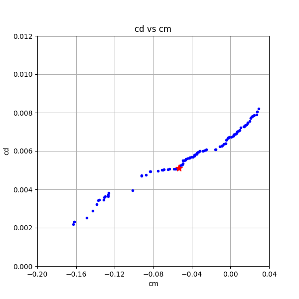
あらためて、パレート解をcd vs cmでプロットすると以下のようになる
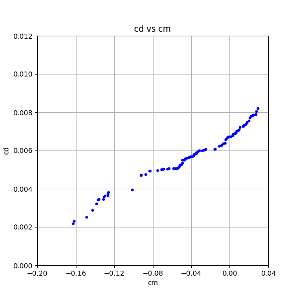
せっかくなので、パレート解のうち以下の翼型を本家XFLR5で解析してみる
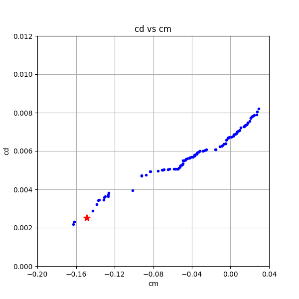
- cd最小あたりのもの(mod2)
- 真ん中の踊り場の中でcm最小のもの(mod29)
- cm最小のグループのうち、cd最小のもの(mod57)
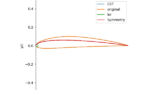
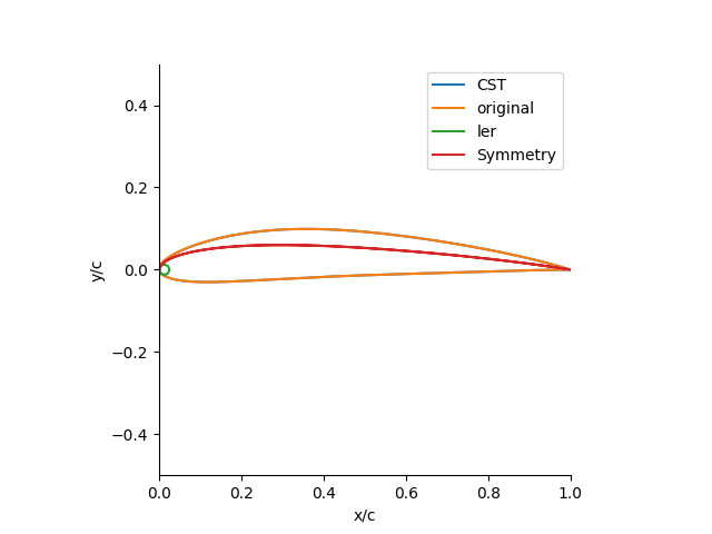
翼型はこんな感じ
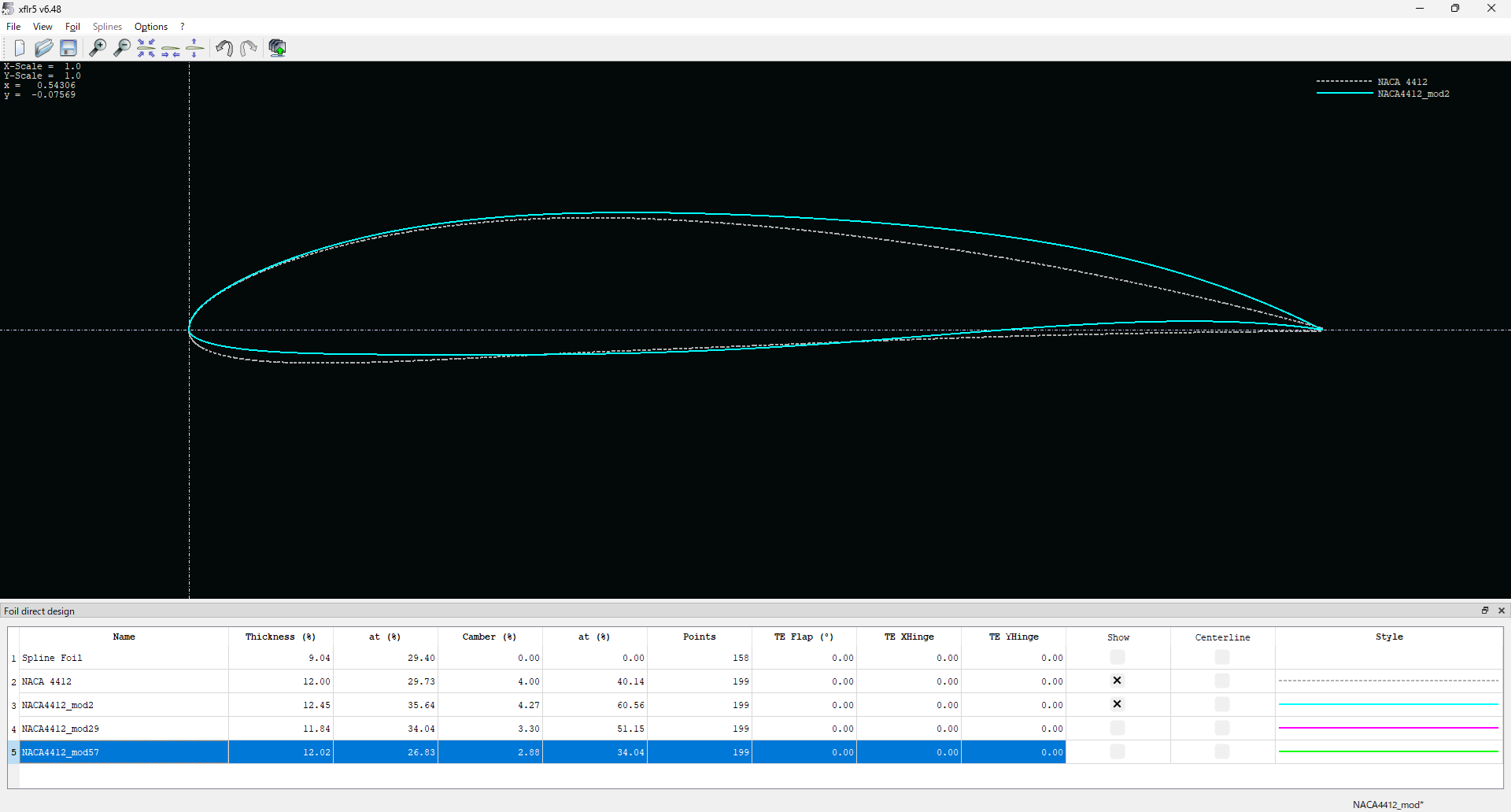
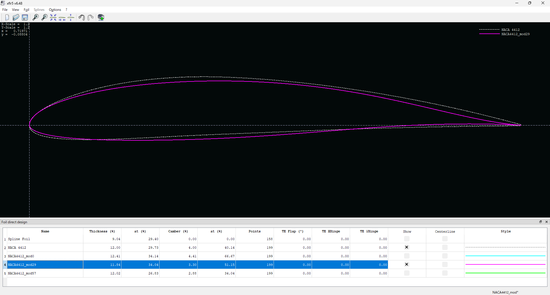
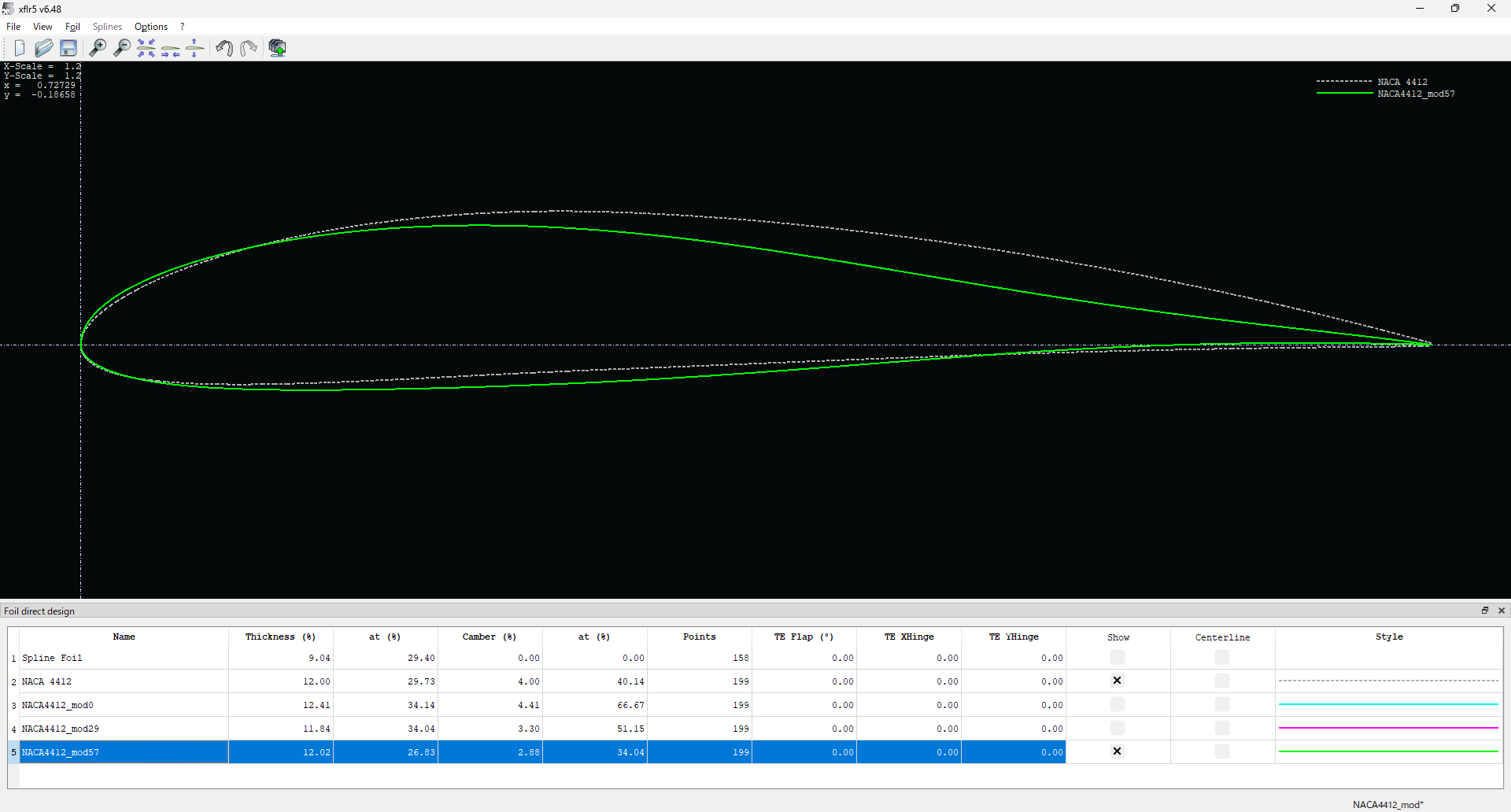
それぞれの性能を計算してみるとこんな感じになる
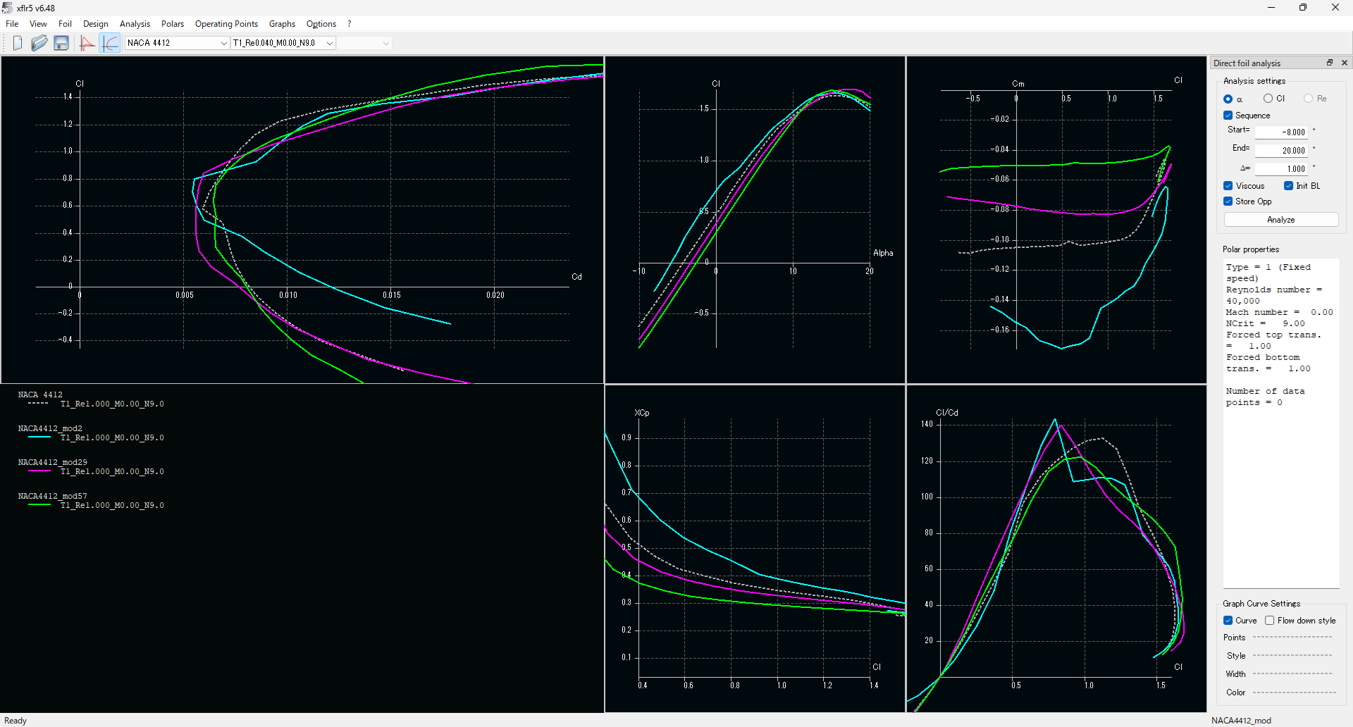
前縁半径や前縁の形に制約を付けたおかげでどれも失速特性は悪くない
Cmの小ささはさすがにmod57が圧勝だが、cdの小ささに関してはmod2よりもmod29のほうがいい感じに見える
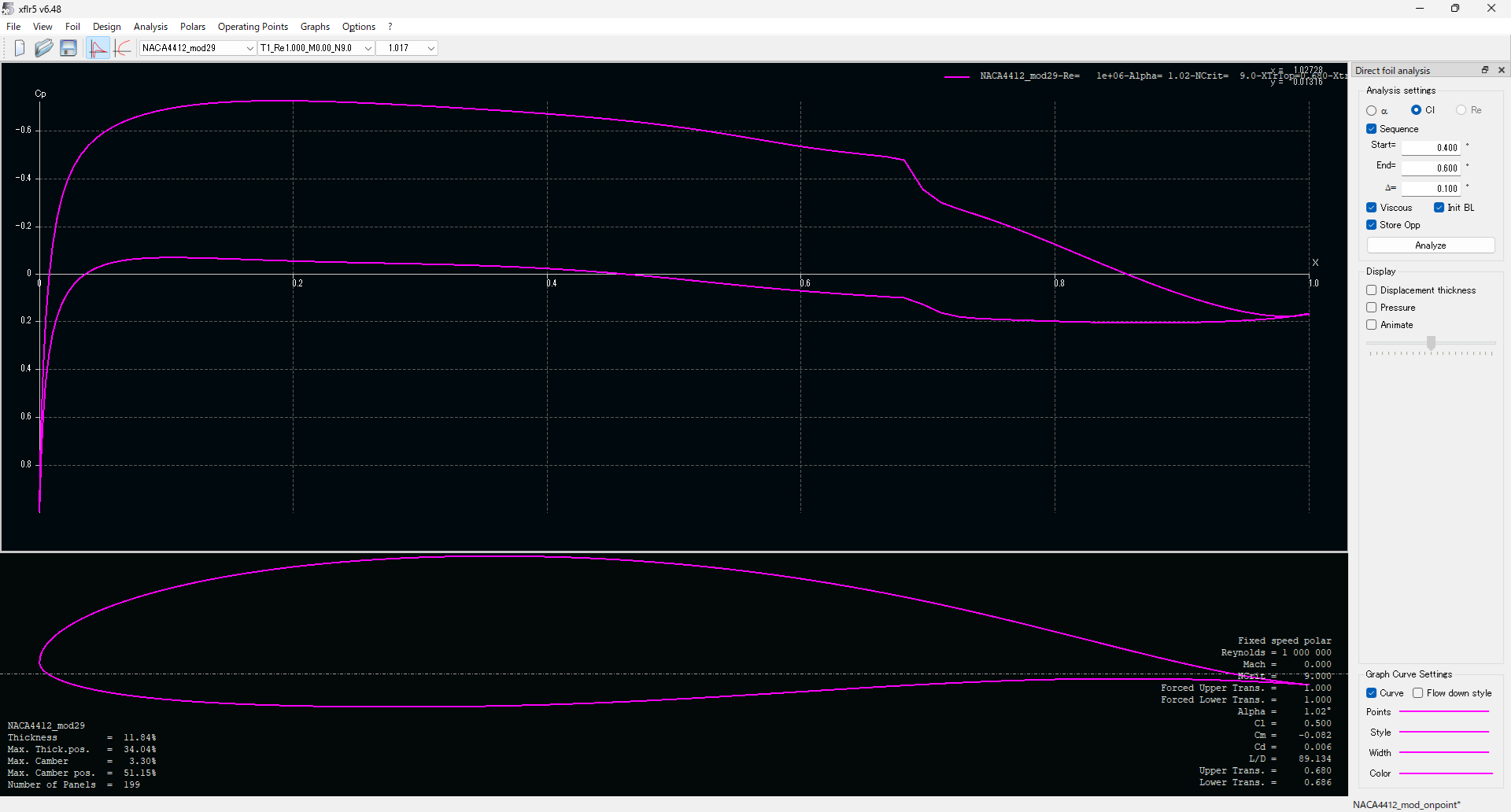
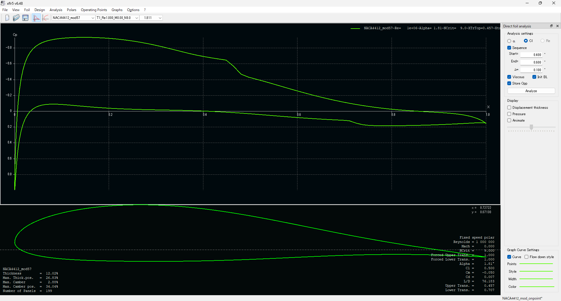
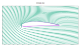
圧力分布はこんな感じ
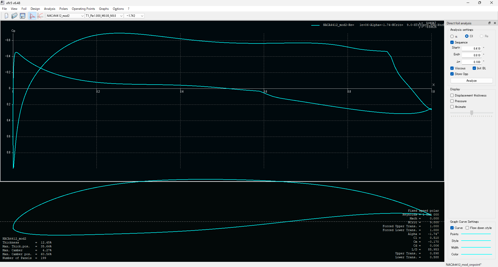
mod2はキャンバーを大きくしてほぼDesign Lift Coefficitnに近いんじゃなかろうかと思う
以上
おわりに
pymooのNSGA-IIとxfoilでCST Airfoilの多目的最適化を行った
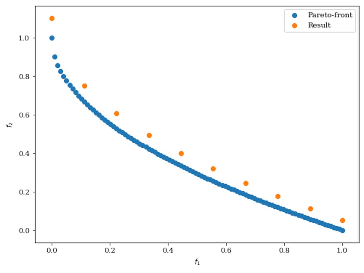
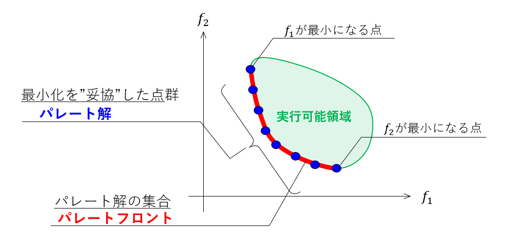
パレート解の存在によって複数の目的関数のトレードオフが目に見えるようになり、なぜその設計を選んだのかの根拠が説明しやすくなる
pythonとChatGPTのおかげでさくさくコードが書けるようになったので、これからいろいろなものを最適化にぶち込んでみようと思う
↓関連記事

おまけ:check.pyの解説
このプログラムは、翼型形状の最適化結果を可視化するためのアニメーションGIFを生成し、目的空間のプロットを表示する
具体的には、CSTクラスを用いて翼型の形状を生成し、最適化結果を読み込み、プロットとアニメーションを作成する
インポート
from CST import CST

import sys
import numpy as np
import pandas as pd
import matplotlib.pyplot as plt
import matplotlib.animation as animationCST: 翼型形状の生成と操作を行うクラス。sys: システム固有のパラメータや関数にアクセスするためのモジュール。numpy: 数値計算をサポートするライブラリ。pandas: データ操作と解析のためのライブラリ。matplotlib.pyplot: プロット作成のためのライブラリ。matplotlib.animation: アニメーション作成のためのライブラリ。
gif_animation( )
GIFアニメーションを作成する
def gif_animation(res, airfoil):
    """
    GIFアニメーションを作成する関数
    Args:
    - res: 最適化結果のデータフレーム
    - airfoil: 翼型形状データ
    """
    fig, (ax_left, ax_right) = plt.subplots(1, 2, figsize=(12, 6))  # 左右に2つのプロットを持つ図を作成

    def _update(i):
        _update_left(i, ax_left, res, airfoil)  # 左側のプロットを更新
        _update_right(i, ax_right, res)  # 右側のプロットを更新

    ani = animation.FuncAnimation(fig, _update, interval=100, frames=len(res), repeat_delay=2000)  # アニメーションを作成

    # 保存
ani.save("./MDO/sample.gif", writer="pillow") # アニメーションをGIFとして保存引数:
res: 最適化結果のデータフレーム。airfoil: 翼型形状データ。
処理:
- 左右に2つのプロットを持つ図を作成する
- アニメーションを更新するための内部関数
_updateを定義する - アニメーションを作成し、GIFファイルとして保存する
_update_left( )
.gifの左側のプロットを更新する
def _update_left(i, ax_left, res, airfoil):
    """
    左側のプロットを更新する関数
    Args:
    - i: 現在のフレーム番号
    - ax_left: 左側のプロットの軸オブジェクト
    - res: 最適化結果のデータフレーム
    - airfoil: 翼型形状データ
    """
    ax_left.clear()  # 現在描写されているグラフを消去
    ax_left.set_title("cd = {:.4f} cm = {:.4f}".format(res['cd'].iloc[i], -res['cm'].iloc[i]))  # タイトルに現在のcdとcmの値を表示
    ax_left.set_xlim(0, 1)  # x軸の範囲を設定
    ax_left.set_ylim(-0.5, 0.5)  # y軸の範囲を設定
ax_left.plot(airfoil.x[i], airfoil.y[i], color='blue') # 翼型形状をプロット引数:
i: 現在のフレーム番号。ax_left: 左側のプロットの軸オブジェクト。res: 最適化結果のデータフレーム。airfoil: 翼型形状データ。
処理:
- 現在のプロットを消去する
- タイトルを更新する(現在の
cdとcmの値を表示) - プロットの範囲を設定する
- 翼型形状をプロットする
_update_right( )
.gifの右側のプロットを更新する
def _update_right(i, ax_right, res):
    """
    右側のプロットを更新する関数
    Args:
    - i: 現在のフレーム番号
    - ax_right: 右側のプロットの軸オブジェクト
    - res: 最適化結果のデータフレーム
    """
    ax_right.clear()  # 現在描写されているグラフを消去
    ax_right.set_title('cd vs cm')  # タイトルを設定
    ax_right.set_ylim(0, 0.012)  # y軸の範囲を設定
    ax_right.set_xlim(-0.1, 0.02)  # x軸の範囲を設定
    ax_right.set_xticks([-0.20, -0.16, -0.12, -0.08, -0.04, 0.00, 0.04])  # x軸のメモリを設定
    ax_right.set_ylabel('cd')  # y軸のラベルを設定
    ax_right.set_xlabel('cm')  # x軸のラベルを設定
    ax_right.grid()  # グリッドを表示
    ax_right.plot(-res['cm'], res['cd'], '.', color='blue')  # cd vs cmのプロット
ax_right.plot(-res['cm'].values[i], res['cd'].values[i], '*', color='red', markersize=10) # 現在のフレームのデータを強調表示引数:
i: 現在のフレーム番号。ax_right: 右側のプロットの軸オブジェクト。res: 最適化結果のデータフレーム。
処理:
- 現在のプロットを消去する
- タイトルを設定する
- 軸の範囲とラベルを設定する
- グリッドを表示する
cdとcmのプロットを更新する- 現在のデータのプロットを★で強調表示する
objective_space( )
目的空間のプロットを表示する
def objective_space(res):
    """
    目的空間のプロットを表示する関数
    Args:
    - res: 最適化結果のデータフレーム
    """
    fig = plt.figure(figsize=(6, 6))  # 図のサイズを指定して作成

    plt.title('cd vs cm')  # タイトルを設定
    plt.ylabel('cd')  # y軸のラベルを設定
    plt.xlabel('cm')  # x軸のラベルを設定
    plt.ylim(0, 0.012)  # y軸の範囲を設定
    plt.xlim(-0.20, 0.04)  # x軸の範囲を設定
    plt.xticks([-0.20, -0.16, -0.12, -0.08, -0.04, 0.00, 0.04])  # x軸の目盛りを設定
    plt.grid()  # グリッドを表示
    plt.plot(-res['cm'], res['cd'], '.', color='blue')  # cd vs cmのプロット

    # 表示
plt.show() # プロットを表示引数:
res: 最適化結果のデータフレーム。
処理:
- 図を作成する
- 軸の範囲とラベルを設定する
- グリッドを表示する
cdとcmのプロットを作成する- プロットを表示する
__main__
最適化結果の読み込みと前処理
res_X = pd.read_csv('./MDO/res_X.csv')
res_F = pd.read_csv('./MDO/res_F.csv')

res = pd.concat([res_X, res_F], axis=1)
res = res.sort_values('cd')
res_np = res.to_numpy()- CSVファイルから最適化結果を読み込む
- 読み込んだデータを結合し、
cdでソートする - データをNumPy配列に変換する
翼型形状の生成
airfoil = CST()
wu = res_np[:, :6].tolist()
wl = res_np[:, 6:].tolist()
dz = np.zeros(len(wu)).tolist()
airfoil.create_airfoil(wu=wu, wl=wl, dz=dz, Node=100)CSTクラスのインスタンスを作成する- 最適化結果から翼型の上面および下面の形状データを抽出する
- 翼型形状を生成する
目的空間のプロット表示とGIFアニメーションの作成
objective_space(res)
gif_animation(res, airfoil)- 目的空間のプロットを表示する
- GIFアニメーションを作成し、保存する
以上
コメント