一般的な移流拡散方程式を有限体積法によって離散化する方法について説明する
keyword: 偏微分方程式の離散化,有限体積法,移流拡散方程式
有限体積法
有限体積法は次のような特徴を持つ離散化手法である
- 積分型の流れの方程式を基礎とする
- 速度や圧力などの物理量は検査体積(セル)の代表値を求める
- 質量や運動量などの保存則はセルの境界からの流入/流出およびセル内部での発生/消滅によって表す
- 非構造格子を用いる
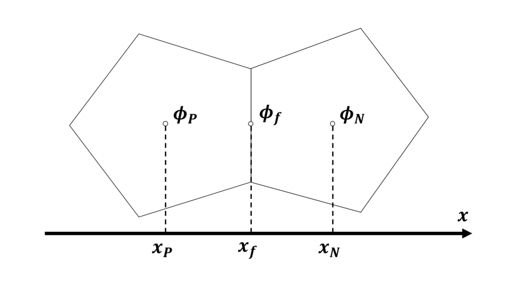
セルが不規則に配置されている非構造格子では,離散化に使える値は注目セル\(P\)の代表値\(\phi_{_{P}}\)と隣接セル\(N\)の代表値\(\phi_{_{N}}\)の2つのみである
2つのセルの間にある境界面\(f\)の代表値\(\phi_{f}\)は\(\phi_{_{P}}\)と\(\phi_{_{N}}\)を用いた補間によって求められる
一般的な輸送方程式に対する離散化
一般に,物理量\(\phi\)の輸送方程式は時間項,対流項,粘性項,ソース項(生成項+散逸項)から構成され,次のようにあらわされる
\begin{equation}
\frac{\partial}{\partial t}(\rho\phi)
+\nabla\cdot(\rho\mathbf{u}\phi)
=s
+\nabla\cdot\left(\Gamma\nabla \phi\right)
\end{equation}
ここで,
- \(\phi=\mathbf{u}\),\(\Gamma=\mu+\mu_{t}\),\(s=-\frac{\partial p}{\partial x}\)とすればNavier-Stokes方程式
- \(\phi=k\),\(\Gamma=\mu+\frac{\mu_{t}}{\sigma_{k}}\),\(s=P_{k}-\varepsilon\)とすれば標準k-εモデルの\(k\)の輸送方程式,
- \(\phi=\varepsilon\),\(\Gamma=\mu+\frac{\mu_{t}}{\sigma_{\varepsilon}}\),\(s=\left(C_{\varepsilon_{1}}P_{k}-C_{\varepsilon_{2}}\varepsilon\right)\frac{\varepsilon}{k}\)とすれば標準k-εモデルの\(\varepsilon\)の輸送方程式
である
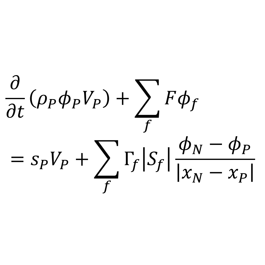
上記の輸送方程式をセル体積で積分し,離散化すると次のようになる
\begin{equation}
\frac{\partial}{\partial t}(\rho_{_{P}}\phi_{_{P}}V_{_{P}})
+\sum_{f}{F\phi_{f}}
=s_{_{P}}V_{_{P}}
+\sum_{f}{\Gamma_{f}\left|S_{f}\right|\frac{\phi_{_{N}}-\phi_{_{P}}}{|\mathbf{x}_{_{N}}-\mathbf{x}_{_{P}}|}}
\end{equation}
また,\(\phi\)の発散と勾配を有限体積法で離散化すると次のようになる
\begin{align}
\nabla\cdot\phi \quad &\rightarrow \quad \sum_{f}\mathbf{S}_{f}\cdot\phi_{f} \\ \\
\nabla\phi \quad &\rightarrow \quad \sum_{f}\mathbf{S}_{f}\phi_{f} \\
\end{align}
ここで,\(V_{_{P}}\)はセル体積,\(|S_{f}|\)は注目セルと隣接セルの境界面の面積,\(\mathbf{S}_{f}\)は境界面に垂直で境界面の面積\(|S_{f}|\)を大きさに持つ法線ベクトルであり,\(\sum_{f}\)はセルがもつすべての面に対する総和を表す
上記3つの離散化を見てみると未知数は\(\phi_{f}\)のみであり,有限体積法の離散化は「境界面上の代表値\(\phi_{f}\)をどのように補間するか」という点に集約されていることがわかる
有限差分法の離散化は微分を「差分」で表し,有限体積法の離散化は微分を「補間」で表すことが両者の大きな違いの1つである
導出
有限体積法は速度や圧力などの物理量を検査体積(セル)の代表値として求めるので,\(\phi\)についての輸送方程式をセル\(P\)について体積積分する
\begin{equation}
\int_{V}{\frac{\partial}{\partial t}(\rho\phi)}dV
+\int_{V}{\nabla\cdot(\rho\mathbf{u}\phi)}dV
=
\int_{V}{s}dV
+\int_{V}{\nabla\cdot\left(\Gamma\nabla \phi\right)}dV
\end{equation}
上式の各項の積分について離散化を行う
ちなみに,ここからの式変形ではガウスの発散定理を多用する
\begin{equation}
\int_{V}{\nabla\cdot\phi}dV=\int_{S}{d\mathbf{S}\cdot\phi}
\end{equation}
参考
≫ガウスの発散定理・ストークスの定理の証明 _ 高校数学の美しい物語
対流項(convection term)
ガウスの発散定理より,対流項は次のように離散化される
\begin{equation}
\int_{V}{\nabla\cdot(\rho\mathbf{u}\phi)}dV
=\int_{S}{d\mathbf{S}\cdot(\rho\mathbf{u}\phi)}
=\sum_{f}{\mathbf{S}_{f}\cdot(\rho\mathbf{u})_{f}\phi_{f}}
=\sum_{f}{F\phi_{f}}
\end{equation}
ここで,\(F=\mathbf{S}_{f}\cdot(\rho\mathbf{u})_{f}\)は質量流束である
対流項は\(\mathbf{u}\)と\(\phi\)という2つの変数の積で表される非線形項であり,離散化に対して最も慎重になる必要がある項である
拡散項
ガウスの発散定理より,対流項は次のように離散化される
\begin{equation}
\int_{V}{\nabla\cdot\left(\Gamma\nabla \phi\right)}dV
=\int_{S}{d\mathbf{S}\cdot(\Gamma\nabla\phi)}
=\sum_{f}{\Gamma_{f}\mathbf{S}_{f}\cdot(\nabla\phi)_{f}}
\end{equation}
ここで,\(\mathbf{S}_{f}\cdot(\nabla\phi)_{f}\)は中心差分を用いて次のように計算される
\begin{equation}
\mathbf{S}_{f}\cdot(\nabla\phi)_{f}
=|S_{f}|\frac{\phi_{_{N}}-\phi_{_{P}}}{|\mathbf{x}_{_{N}}-\mathbf{x}_{_{N}}|}
\end{equation}
ソース項(Source terms)
ソース項は次の3つの条件に応じて計算の仕方が異なる
- ソース項が既知の変数を用いて陽的に計算できる
- ソース項の中に変数\(\phi\)が入っており,係数\(\rho\)が正である
- ソース項の中に変数\(\phi\)が入っており,係数\(\rho\)が負である
(1)の場合は,注目セルにおける代表値を用いて直接計算できる
\begin{equation}
\int_{V}{s}dV
=s_{_{P}}V_{_{P}}
\end{equation}
(2)と(3)の場合は,係数行列\(\mathbf{A}_{p}\)の対角優位性を保って計算の安定性を高めるために,係数\(\rho\)の符号によって計算方法を切り替える(係数行列の対角成分が大きくなると計算が安定する)
(2)の場合は,ソース項を陰的に計算して係数行列の対角成分を大きくする
\begin{align}
&\int_{V}{\rho\phi}dV=\rho_{_{P}}V_{_{P}}\phi_{_{P}} \\
\\ \rightarrow \quad
& \mathbf{A}_{_{P}}\phi_{_{P}}
+\mathrm{max}\left(\rho_{_{P}},0\right)V_{_{P}}\phi_{_{P}}
=\left\{\mathbf{A}_{_{P}}+\mathrm{max}\left(\rho_{_{P}},0\right)V_{_{P}}\right\}
\phi_{_{P}}
\end{align}
(3)の場合は,ソース項を陽的に計算する
\begin{align}
\int_{V}{\rho\phi}dV=\rho_{_{P}}V_{_{P}}\phi_{_{P}}
=\mathrm{min}\left(\rho_{_{P}},0\right)V_{_{P}}\phi_{_{P}}
\end{align}
参考
≫ヤコビ法,ガウス・ザイデル法の 収束条件と対角優位性(PDF)
3.4.9 Source terms
Source terms can be specified in 3 ways
Explicit Every explicit term is a volField. Hence, an explicit source term can be incorporated into an equation simply as a field of values. For example if we wished to solve Poisson’s equation \(\nabla^{2}\phi=f\), we would define phi and f as volScalarField and then do\begin{equation}
\mathrm{solve(fvm::laplacian(phi) == f)}
\end{equation}Implicit An implicit source term is integrated over a control volume and linearised by
\begin{equation}
\int_{V}{\rho\phi}dV=\rho_{_{P}}V_{_{P}}\phi_{_{P}}
\end{equation}Implicit/Explicit The implicit source term changes the coefficient of the diagonal of the matrix. Depending on the sign of the coefficient and matrix terms, this will either increase or decrease diagonal dominance of the matrix. Decreasing the diagonal dominance could cause instability during iterative solution of the matrix equation. Therefore OpenFOAM provides a mixed source discretisation procedure that is implicit when the coefficients that are greater than zero, and explicit for the coefficients less than zero. In mathematical terms the matrix coefficient for node P is \(V_{_{P}}\mathrm{max}\left(\rho_{_{P}}, 0\right)\) and the source term is \(V_{_{P}}\phi_{_{P}}\mathrm{min}\left(\rho_{_{P}}, 0\right)\).
OpenFOAM Programmar's Guide p.43
発散(Divergence)
ガウスの発散定理より,発散は次のように離散化される
\begin{equation}
\int_{V}{\nabla\cdot\phi}dV
=\int_{S}{d\mathbf{S}\cdot\phi}
=\sum_{f}{\mathbf{S}_{f}\cdot\phi_{f}}
\end{equation}
輸送方程式の一般形には含まれていないが,
- \(\phi=\nu_{e}\left(\nabla\mathbf{u}\right)^{T}\)とすれば Navier-Stokes方程式の粘性項の片割れ
- \(\phi=\mathbf{N}=\tau_{ij}^{a}-(-2\nu_{t}S_{ij})\)とすれば外力項として実装される乱流応力の非線形項
である
勾配(Gradient)
ガウスの発散定理より,勾配は次のように離散化される
\begin{equation}
\int_{V}{\nabla\phi}dV
=\int_{S}{d\mathbf{S}\phi}
=\sum_{f}{\mathbf{S}_{f}\phi_{f}}
\end{equation}
輸送方程式の一般形には含まれていないが,\(\phi=-\frac{1}{\rho}p\)とすれば Navier-Stokes方程式の圧力項である
時間項
時間項は次のように計算できる
\begin{equation}
\int_{V}{\frac{\partial}{\partial t}(\rho\phi)}dV
=\frac{\partial}{\partial t}(\rho_{_{P}}\phi_{_{P}}V_{_{P}})
\end{equation}
時間項は陰解法によって離散化される
連立方程式
上記の離散化を行うと,一般的な輸送方程式は次のようにあらわされる
\begin{equation}
\frac{\partial}{\partial t}(\rho_{_{P}}\phi_{_{P}}V_{_{P}})
+\sum_{f}{F\phi_{f}}
=s_{_{P}}V_{_{P}}
+\sum_{f}{\Gamma_{f}\left|S_{f}\right|\frac{\phi_{_{N}}-\phi_{_{P}}}{|\mathbf{x}_{_{N}}-\mathbf{x}_{_{P}}|}}
\end{equation}
時間項に陰解法を用いて離散化し,\(\phi_{_P}\)と\(\phi_{_N}\)を用いて\(\phi_{f}\)を補間すると,次のような連立方程式が得られる
\begin{equation}
\mathbf{A}_{_P}\phi_{_P}+\sum{\mathbf{A}_{_N}\phi_{_N}}
=\mathbf{b}_{_P}
\end{equation}
この連立方程式を反復法で解けば,輸送方程式の解が求められる
まとめ
流れの基礎方程式である連続の式とNavier-Stokes方程式を有限体積法によって離散化する方法について説明した
非構造格子で離散化に使える値は,注目セル\(P\)の代表値\(\phi_{_{P}}\)と隣接セル\(N\)の代表値\(\phi_{_{N}}\)の2つのみである
有限体積法による離散化は「境界面上の代表値\(\phi_{f}\)をどのように補間するか」という点に集約されている
↓具体的な離散化手法はこちら
↓おすすめ記事


コメント